Основы Maple

Robert M. Corless
Department of Applied Mathematics
University of Western Ontario
London, Canada

Copyright 2001 by Robert M. Corless
All rights reserved

Useful one-word commands

Использование монокоманд

Solving equations

Решение уравнений

dsolve

Команда dsolve

> restart;

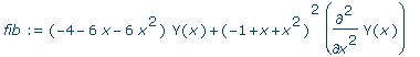
>fib := (-4-6*x-6*x^2)*Y(x)+(-1+x+x^2)^2*diff(Y(x),x,x);

>Order := 14;

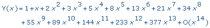
> dsolve( {fib,Y(0)=1,D(Y)(0)=1}, Y(x), series );

> seq(combinat[fibonacci](n),n=1..14);

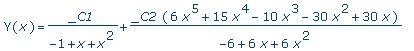
> dsolve( fib, Y(x) );

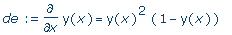
>de := diff(y(x),x) = y(x)^2*(1-y(x));

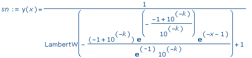
>sn := dsolve({de,y(0)=10^(-k)},y(x));

> plot3d(rhs(sn),x=0..10^3,k=0..3,axes=BOXED);

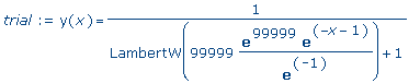
>trial := eval(sn,k=5);

> plot(rhs(trial),x=0.999e5..1.001e5);

> restart;

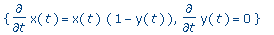
>dsys := {diff(x(t),t)=x(t)*(1-y(t)), diff(y(t),t)=s*y(t)*(x(t)-1) };

In the text, this line has dsys[1] and dsys[2] in it; but this violates one of the "Worksheet Hygiene" rules, and indeed the dysys set may be in a different order. So for this worksheet I have modified the command to use a substitution to get it right. This also makes the text shorter and more intelligible, too.

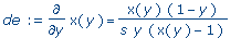
>de := diff(x(y),y) = subs( x(t)=x(y), y(t)=y, subs(dsys,diff(x(t),t)/diff(y(t),t)) );

> _EnvAllSolutions := true;

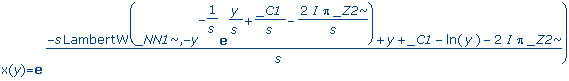
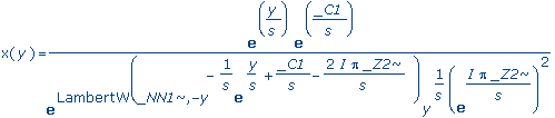
> dsolve(de,x(y));

> expand(%);

> simplify(%);

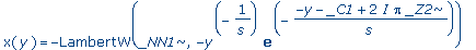
> subs(_Z2=0,%);

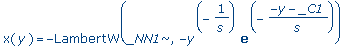
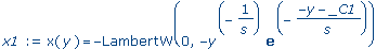
>x1 := subs(_NN1=0,%);

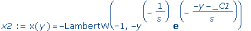
>x2 := subs(_NN1=-1,%%);

>s := rand()/1.0e12;

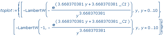
>toplot := {[rhs(x1),y,y=0..10],[rhs(x2),y,y=0..10]};

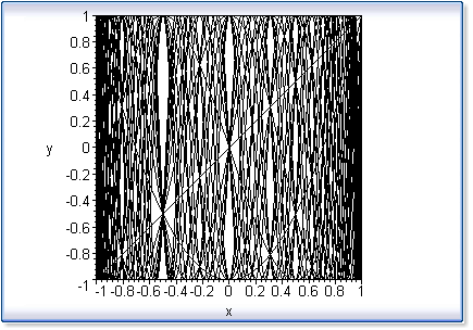
>sols := `union`(seq(toplot,_C1={-7,-6,-5,-4,-3,-2,-3/2,-1-s})):

> plot(%,view=[0..20,0..10],colour=black);

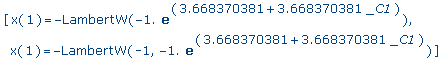
> eval([x1,x2],y=1);

> subs(_C1=-1-s,%);

> evalf(%);

>s := 's';

> solve(X1 = rhs(eval(x1,y=1)), _C1);

> subs(_Z5=0,%);

> subs(s=0,dsys);

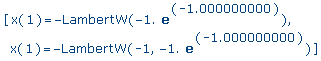
> dsolve(%,{x(t),y(t)});

$[{y(t) = _C2}, {x(t) = _C1*exp(Int(1-y(t),t))}]$

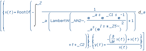
> dsolve(dsys,{x(t),y(t)});

$[{x(t) = 0}, {y(t) = _C1*exp(-s*t)}], [{x(t) = Root...$

> restart;

> plots[setoptions](colour=BLACK);

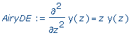
>AiryDE := diff(y(z),z,z) = z*y(z);

> dsolve( AiryDE, y(z) ) ;

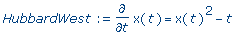
> HubbardWest := diff(x(t),t) = x(t)^2 - t;

> dsolve( HubbardWest, x(t) );

> dsolve( {HubbardWest, x(0)=alpha}, x(t) );

>X := rhs( % ):

>Nplot := 10;

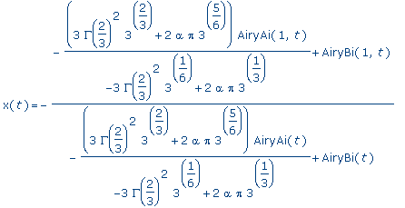
>P := plot( [seq(X,alpha=[seq(-5*i/Nplot, i=0..Nplot)])],t=0..8, y=-5..0,
scaling=CONSTRAINED ): plots[display](P);

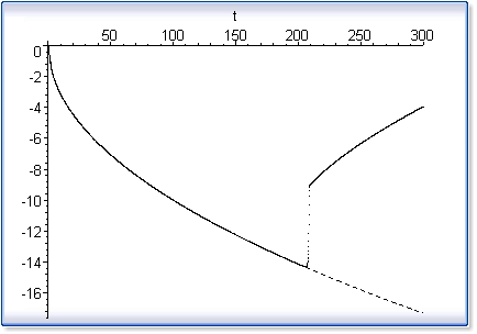
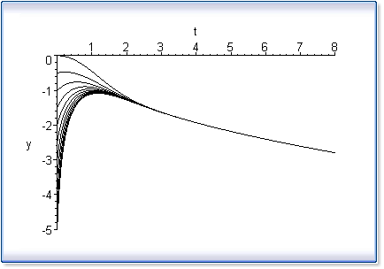
>P1 := plot( eval(X,alpha=0), t=0..300, linestyle=4 ): plots[display](P1);

>N := 3000;

>h := 300.0/N;

>badsol := dsolve({HubbardWest,x(0)=0},numeric,method=classical[rk4], stepsize=h,output=procedurelist);

> wrongpts := [seq( subs( badsol(k*h),[t,x(t)]), k=0..N)]:

>P2 := plot( wrongpts, style=POINT, colour=black, symbol=POINT ):

> plots[display]({P1,P2});

> goodsol := dsolve( {HubbardWest,x(0)=0}, numeric, stiff=true, range=0..1.0e8 );

> plots[odeplot]( goodsol, style=POINT, symbol=POINT, colour=BLACK );

> goodsol( 1.0e5 );

>eval( X, [alpha=0, t=1.0e5] );

>evalf( % );

> goodsol( 1.0e7 );

>-sqrt( 1.0e7 );

>eval( X, [alpha=0, t=1.0e7] );

> goodsol( 1.0e8 );

>-sqrt( 1.0e8 );

Multiple paths from the same equation

> restart;

>Suzen := proc (m, t, yvec, ypvec) local i, j;
option `[yvec[1] = x(t), yvec[2] = diff(x(t),t),
yvec[3] = y(t), yvec[4] = diff(y(t),t)]`;
for i to m/4 do
j := 4*(i-1);
ypvec[1+j] := yvec[2+j];
ypvec[2+j] := -yvec[1+j]^2+yvec[3+j]^2;
ypvec[3+j] := yvec[4+j];
ypvec[4+j] := 2*yvec[1+j]*yvec[3+j];
end do;
ypvec
end proc:

>N := 72;

>ic := map(evalf,vector( 4*N, [seq(op([cos(2*Pi*(i-1)/N),0,sin(2*Pi*(i-1)/N),0]),i=1..N)])):

>pvars := [seq(z||i(t),i=1..4*N)]:

>st := time(): sol := dsolve( numeric, procedure=Suzen, range=0..3, start=0, initial=ic, procvars=pvars ):
time_taken_de := time() - st;

Warning, cannot evaluate the solution further right of 2.9744778, probably a singularity

>st := time(): plots[odeplot]( sol, [seq([z||(1+4*(i-1))(t),z||(3+4*(i-1))(t)],i=1..N)], colour=black, view=[-3..3,-3..3], scaling=CONSTRAINED, labels=["",""], axes=BOXED );
time_taken_plotting := time() - st;

> time_taken_plotting/time_taken_de;

С официального разрешения © 2002 Waterloo Maple, Inc