Пусть , x = 2, и x = 0.4.

Вычислить y, dy, построить график функции f(x) и касательную при x = 2.

> restart:

> f:= x -> x^5;

> D(f);

> f( 2 + 0.4) - f(2);

> f(2.4);

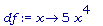
> df:= x -> 5*x^4;

> df(2);

> 80 * .4;

Следовательно, y = и dy = f '(2) (0.4) = 32;

заметим при этом, что x = 0.4 всё-таки великовато.

> tl:= x -> 32 + 80*(x - 2);

> tl(2.4);

> with(plots):

> A:= plot({f(x),tl(x)}, x= 1.5..2.7, color=[blue,brown]):

> B:= plot([t,32,t = 2..2.4], color = magenta):

> C:= plot([2.4,t,t= 32 ..79.62624], color = magenta):

> F:= plot([t, 64, t= 2.4..2.6], color = black):

> G:= plot([2.6,t,t=64..79.62624], color = black):

> H:= plot([t,79.62624, t= 2.4..2.6], color = black):

> K:= textplot([2.65,74,'dy'],color = red):

> L:= textplot([2.5,50,'deltay'] , color = red):

> M:= textplot([2.2,20,'deltax'],color = red):

> display({A,B,C,F,G,H,K,L,M}, axes = boxed);

Можно утверждать, что касательная - линейная аппроксимация функции. Мы в этом примере увидели, что при больших

x , линейная аппроксимация НЕ является хорошей.